Imagine a machine that can transform what enters it into a point in a higher-dimensional space.  

   Sounds crazy? Well, we can do that for classification and regression analysis with a mathematical model called Support Vector Machines (SVMs).

Introduction

     SVMs are models for supervised learning that has been around since the early ’60s. It got a lot of improvements over time and became a method recognized for its performance and reliability and still plays a significant role in machine learning/computer vision today.

   Our amazing friend, OpenCV, has an implementation of SVM in its contrib modules (to know how to install the OpenCV with contrib modules, please see my tutorial).

   Support Vector Machines are an extensive topic; here I’ll explain the basic concepts, just not to implement it without actually knowing what it does. So by the end of this post, you will be capable of understanding how it works and even implementing one yourself.

How does SVM works?

     Let’s suppose a classification problem, containing two very distinct classes, as shown in Figure 1.

Figure 1 – A two-class classification problem

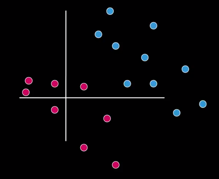
     For acceptably doing the classification,  in that case, the classes must be in different parts of a spectrum. So, we can separate the pinks from the blues easily with a line. Look at Figure 2.

Figure 2 – Classes separated by a line

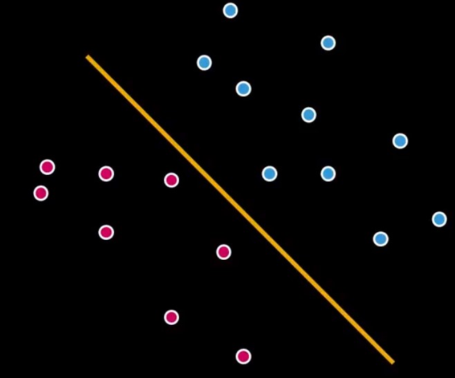
     Now we have a type of classifier called Linear Classifier. But actually, there’s a lot of different ways we can draw that line, see more in Figure 3.

Figure 3 – Other possibilities

The SVM approach

     All lines from Figure 3 separate the pinks and the blues. Considering all possibilities only one line could be the best, but which one? That is where SVMs come to place. SVMs are the machinery programmed to search for the best possible separation line (hyperplane). Look at Figure 4.

Figure 4 – Margins

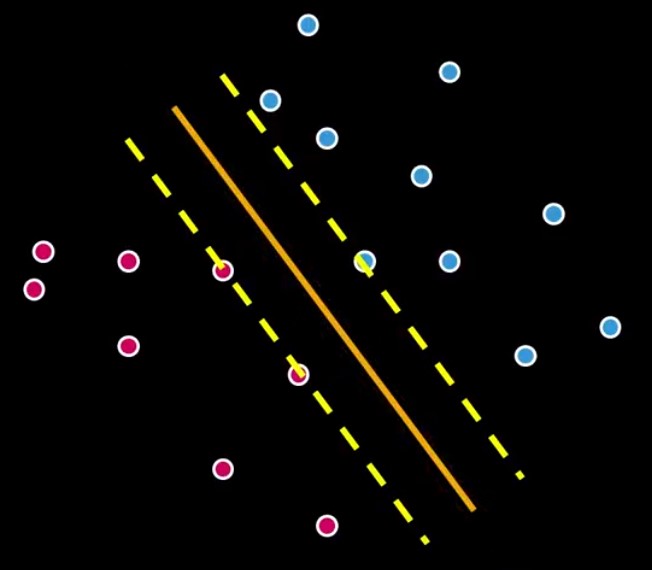
     The two additional dashed lines are the margins. The SVM computes an optimization problem, searching for the greatest possible margin between the hyperplane and any point within the training set.

Non-Linear SVMs

      There are cases where there’s no possible linear separation, as Figure 5 shows.

Figure 5 – Two classes that are impossible to separate with a line

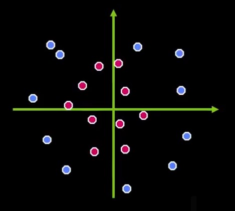
    How about transforming the current space into a higher dimensional one, where the dots also have a depth value. Imagine Figure 5 in a 3-dimensional space. That classification problem might have a plane to separate the classes, like Figure 6.

Figure 6 – The case in Figure 5 is now separable by a plane

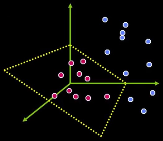
     This works for any n-dimensional problem. SVMs can efficiently handle that with a remarkable simplification. The idea behind is called the “Kernel trick”. Kernels are a similarity function that corresponds to some inner product in some expanded feature space. So, because of it, we don’t need to know the coordinates of the data in that space. This simplifies the calculations and thus, the computing time.

Programming an SVM with OpenCV

     It’s possible to configure, train and use an SVM with OpenCV in less than ten lines of code. There are four main steps to do:  Create the SVM, set its type, the kernel, and the termination criteria.

Creation and parameter definition

     Take a look at the code snippet below.

     Line by line:

1.  Creating the Support Vector Machine using an instance of the class cv::ml::SVM;
2. Definition of the type C_SVC, which means the SVM is ready for an N class classification. To see more types, take a look at the documentation;
3. The Kernel was used to map the data. For most non-linear cases, RBF does a pretty good job. See more options here.
4. Like I said before, SVM training solves an iterative optimization problem. Then, it becomes necessary to define a time for it to stop. Here, we choose the number of iterations and a tolerance value. There are other options described at the documentation.

Training

It’s possible to do training like the snippet below:

  Line 1 creates the training data using OpenCV’s Mat  Matrix. The trainingMatrix variable contains a series of images one per row. So, a little processing is necessary to adapt your images to a training set. The variable labels is also a Mat, containing all image labels.

    Then Line 2 train the SVM. It could take a while, depending on the training set’s size.

    After the training, it is possible to use the command svm->predict  to classify a sample.

    The output must be a value that belongs to one of the classes and…That’s all! Let’s try to identify something using images?

Test case

     I recently discovered the International Skin Imaging Collaboration (ISIC), and its Melanoma Project which is an open-source public access archive of skin images from the International Society for Digital Imaging of the Skin (ISDIS). The Melanoma research project defines the disease as:

     Melanoma is usually, but not always, a cancer of the skin. It begins in melanocytes – the cells that produce the pigment melanin that colors the skin, hair and eyes. (…) Unlike other cancers, melanoma can often be seen on the skin, making it easier to detect in its early stages. If left undetected, however, melanoma can spread to distant sites or distant organs.

     There are some studies applying Support Vector Machines in Melanoma images, like the ones done by Dreiseitl (2001) or Gilmore, Hofmann-Wellenhof, and Soyer (2010). Let’s analyze the images and see what can be done.

The images

     When seen on the skin, the color difference of the lesion is often noticeable, see Figure 7.

Figure 7 – Melanoma lesion

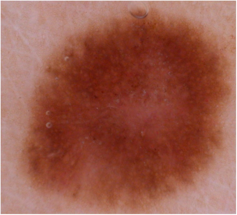
   That makes things fairly easier because of high-frequency components, allowing us to use a good edge-image in training.

     With that in mind I developed an algorithm that can be briefly described in these five steps:

1.  Load the images;
2. Extract the edges using the Sobel Kernel;
3. Transform all images into a vector;
4. Create and train the SVM;
5. Obtain the prediction.

Results

     I selected 26 random images from the database, 13 from benign and 13 malignant lesions. From that, 20 of them were used in the training process and 6 (3 malignant and 3 benign) in the validation.

     All the parameters used were the same as the code snippets above. The SVM achieved the expected values in 100% of the cases, see table 1.

Table 1 – Test values.

     That went way better than I expected. Of course, only 6 validation images is not enough to conclude anything. We could improve the reliability of the training with more test images (papers usually report 80%+ accuracy) and other image features such as HOG. But for now, is enough to understand and ‘feel’ a little of the Support Vector Machines’ power.

     You can test it by yourself (mail me the results 🙂 ), the code and the images are available on my Github page.

PS: All images used here are from Udacity Computer Vision Course.