Convolution is a well-known mathematical operation largely used in image processing for filtering operations. It is also an expensive task for the CPU since it’s an iterative process based on sums and multiplications. So, bigger images, longer processing times.

     To lower its processing times, we can parallelize the task over the available CPU cores. There’s some work in the last years with this approach like Yu et al. (1998), Pande & Chanda (2013), Ström (2016), or even available C implementations at Github.

   I’m currently using Python on a project, so I decided to parallelize the Convolution and evaluate its performance since I couldn’t find anything Python-related or sufficiently conclusive over the internet. This text describes the algorithm and the results of the tests.

A little about convolution

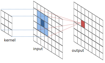
  The convolution is performed by sliding a matrix called Kernel (or Convolution Matrix) over the image, starting on the top left all the way to the bottom right.

     This process will generate an output image in which each pixel will be the sum of all the multiplications of the region where the Kernel is ‘hovering’ on the original image. This entire process is illustrated below as a gif (from Wikipedia).

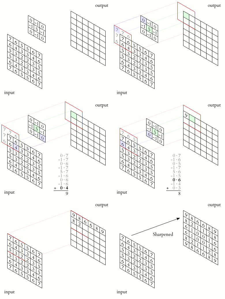
Figure (Gif?) 1 – Step by step of the convolution process.

The implemented algorithm

    Briefly, the Python algorithm I coded can be separated into five steps:

1. Define N as the number of available cores;
2. Slice the input image into (N^2)+2 sub-images;
3. Create the parallel instances;
4. Convolve each sub-image with the desired kernel;
5. Create the output image with the sub-images joining.

 I decided not to implement a new Convolution function, so, I used scipy/numpy built-in solutions (convolve2d() function) and joblib library for parallelization (with Parallel() function).

    The code is available on my Github.

Performance measuring methodology

   For test fidelity, all the time and consumption tests followed the same measurement procedure, which was:

• Execute the code once, then discard the output value;
• Record the time or memory consumption of the next three tests;
• Perform an average of these three values.
• For the time recording, the measurement started a line before the processing began and finished a line after.

     The computer I used had the following settings:

• Processor: I5 3330, 3 GHz;
• Memory: 8 GB DDR3 1333MHz;
• OS: Windows 10 Home x64.

Tests and discussion

Finding the optimization for the slicing procedure

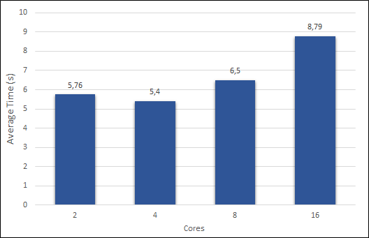
   Before starting, a piece of rather important information is missing: How many processor cores do the algorithm must use to obtain better results? As presented before in the Methodology, the test PC had four cores. A variable in the algorithm depends on that value to slice the image, thus, more cores, more slices. So, I tried to increase the value to see what will come out.

    Figure 2 presents the obtained values, using a 3×3 Sobel Filter and a 225,000,000 pixels image.

Figure 2 – Average time based on the ‘Number of Cores’ value.

     The optimal value appeared when it matched the number of cores in the test PC.

     With the optimal number of cores, I tried to predict the expected gain with Amdahl’s law. Considering that approximately 85% of the algorithm is affected by parallelization, we have a possible time reduction of 2,75 times, as follows:

Time Evaluation

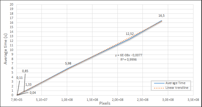
     A total of 7 images were used with resolutions ranging from 1,024×768 to 15,000×15,000 and convolved with a 3×3 Sobel filter. The time values I obtained for the algorithm without parallelization are shown in Figure 3.

Figure 3 – Evaluation of the non-parallelized convolution algorithm.

    The graph presents linear behavior series with a 0.9996 correlation to its trendline. To achieve the given values, the convolve2d() function was used directly, with only the Kernel and the input image.

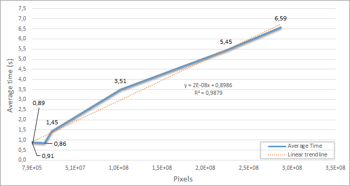
    Figure 4 shows the times’ values from the tests with the parallelized algorithm.

Figure 4 – Evaluation of the parallelized convolution algorithm.

     The behavior is still linear, with a slightly lower correlation, 0.9879. Table 1 shows the graph difference for the parallel and conventional implementation, point by point.

Table 1 – The Point-by-point difference between Figure 3 and 4 graphs.

  It is possible to see with a ~100 million pixels image, the parallel implementation started to overcome the non-parallel.

     Applying Amdahl’s law at point 5, the gain was 1.7 times, on 6, 2.29, and 7, 2.5, which was close to the expected 2.75 theoretical maximum.

Memory evaluation

     Figure 5 shows the algorithm’s maximum memory consumption values for the same images.

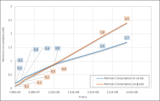
Figure 5 – Memory consumption comparison for the parallelized and non-parallelized convolution algorithms.

     Table 2 shows the point-by-point memory difference.

Table 2 – Point-by-point memory difference of Figure 5 values

    The parallel implementation consumed fewer memory resources when applied to bigger inputs. When it went worse, it never consumed more than a 100MB difference. It is expected behavior since the convolve2d() allocates the entire image for the non-parallelized algorithm. While in the parallelized version, it instantiates, only the sub-images.

Conclusion

     Here, I evaluated a parallel convolution algorithm implemented with the Python language. The parallelization process consists of slicing the image in a series of sub-images followed by the 3×3 filter application on each part and then rejoining the sub-images to create the output.

     On images with more than 100 million pixels, the parallel algorithm took less time and consumed less memory. This shows that parallel convolution using Python is a suitable way for doing faster image filtering.