OpenCV with Python: Thresholding and Masking Explained

Separating What Matters from What Does Not

A lot of computer vision tasks come down to a deceptively simple question: which parts of this image do I care about, and which parts can I ignore? Thresholding and masking are the most direct tools for answering that question. They let you segment an image into regions based on pixel intensity, isolate objects from backgrounds, and focus subsequent processing on exactly the area you need.

These are not flashy techniques, but they are effective and fast. In controlled environments, a well-tuned threshold can replace a much more complex detection pipeline. Even in modern deep learning workflows they still show up regularly in pre and post processing steps.

What Is Thresholding

Thresholding converts a grayscale image into a binary image. Every pixel is compared against a threshold value: pixels above it become white, pixels below it become black, or vice versa depending on the mode. The result is a clean separation between two regions based on brightness.

The underlying idea is simple. If you are trying to read text on a white page, the dark ink pixels and the bright background pixels have very different intensity values. A threshold somewhere in between cleanly separates them. The same logic applies to bright objects on dark backgrounds, lit regions versus shadows, and many other real-world scenarios.

Simple Thresholding

The most basic form applies a single fixed value across the entire image. Everything above the threshold becomes white, everything below becomes black. Like most OpenCV analysis functions, thresholding works on grayscale images, so the first step is always converting from BGR with cv2.cvtColor(image, cv2.COLOR_BGR2GRAY):

The arguments are: the grayscale image, the threshold value, the maximum value to assign to pixels that pass the threshold, and the thresholding type. cv2.THRESH_BINARY sets passing pixels to 255 (white) and the rest to 0 (black). cv2.THRESH_BINARY_INV does the opposite, which is useful when your object of interest is brighter than the background.

cv2.threshold() returns two values: the threshold that was used and the resulting binary image. When you set the threshold manually, the first return value just echoes back what you passed in.

The obvious limitation of simple thresholding is that you have to pick the value yourself, and a fixed value only works well when the lighting across the image is consistent. On images with varying illumination, a single threshold will work well in some areas and poorly in others. You can see both modes applied to the same image below, normal and inverted.

Otsu’s Method

Otsu’s method solves the threshold selection problem automatically. Instead of you picking a value, the algorithm analyzes the histogram of the image and finds the threshold that best separates the two dominant intensity groups. It works by minimizing the weighted variance within each group, and it does it in a single pass over the histogram rather than the image itself, so it is fast.

Passing 0 as the threshold value tells OpenCV to ignore it and let Otsu calculate the optimal one. The + combines two flags: the thresholding type and the Otsu flag. The returned ret value now actually tells you what threshold was chosen, which is useful to know when debugging or logging.

Otsu works best on images with a bimodal histogram, meaning two clear peaks of pixel intensities representing foreground and background. On images where those two groups are not clearly separated in the histogram, the result may not be meaningful. Applying a Gaussian blur before Otsu is also a common practice, it smooths out noise that would otherwise distort the histogram and throw off the calculation. The result with blur applied is shown below:

Adaptive Thresholding

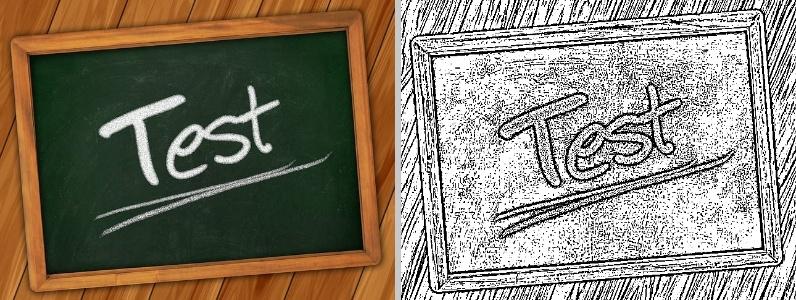
Both methods above apply a single threshold value across the whole image. On images with uneven lighting, like a document photographed under a lamp that is brighter on one side than the other, that falls apart. Adaptive thresholding fixes this by computing a different threshold for each small region of the image independently, based on the local pixel intensities around each point.

The arguments after the image are: the maximum value, the adaptive method, the thresholding type, the block size, and a constant subtracted from the computed threshold. The block size defines how large the local neighborhood is for each pixel, it must be an odd number. The constant C fine-tunes the result: increasing it makes the threshold more aggressive and produces fewer white pixels, decreasing it is more permissive.

cv2.ADAPTIVE_THRESH_GAUSSIAN_C weights the neighborhood pixels by a Gaussian kernel, giving more influence to pixels closer to the center. The alternative is cv2.ADAPTIVE_THRESH_MEAN_C, which treats all neighborhood pixels equally. Gaussian tends to produce smoother, more natural-looking results. Compare the original and the adaptive result below and notice how it handles uneven brightness across the frame.

Masking

A mask is a binary image used to control which pixels in another image are processed or visible. White pixels in the mask mean “include this pixel”, black pixels mean “ignore it”. Applied to an image, the mask zeroes out everything outside the region of interest and leaves the rest untouched.

A common use case is combining a mask derived from thresholding with the original image to isolate the detected region:

cv2.bitwise_and() performs a bitwise AND between two images. When a mask is supplied, only pixels where the mask is 255 are included in the output. Pixels where the mask is 0 become black. The result is the original color image with everything outside the thresholded region removed, as you can see below.

You can also build masks manually without thresholding, for example to define a fixed rectangular or circular region:

Here a blank black mask is created, a filled white circle is drawn on it, and then it is applied to the image. Only the circular region survives, everything else goes black. This pattern, create a mask, draw a shape on it, apply it, shows up constantly when you need to process or display only a specific area. The result below makes it immediately clear how the mask works.

Practical Tips

Thresholding is very sensitive to lighting. If your results are inconsistent across different images of the same subject, the first thing to investigate is whether the lighting conditions are changing. Adaptive thresholding handles variation within a single image, but if the problem is between images, you need consistency at the capture stage.

Always blur before thresholding when working with noisy images. A small Gaussian blur smooths out pixel-level noise that would otherwise create scattered white or black pixels in the binary output, making the result much cleaner and easier to work with downstream.

Otsu is a good default when you do not know the threshold upfront, but do not assume it will always work. Check the output visually. On images with complex or multimodal histograms, the threshold it picks can be far from useful and you will need to fall back to manual values or adaptive thresholding instead.

Wrapping Up

Thresholding and masking are among the most practical tools in the OpenCV toolkit. They are fast, simple to reason about, and effective in the right conditions. In controlled settings a good threshold can do a lot of the heavy lifting that people assume requires something more sophisticated.

The key is knowing their limitations: they work on intensity, so color and texture are invisible to them, and they struggle when lighting is uneven or the foreground and background intensities overlap. When those conditions are met, reach for something else. When they are not, these tools will get you most of the way there with very little code.

Check out the other articles in this series:

1. Installation, Setup, and Your First Computer Vision Program
2. How Images Are Represented in Computer Vision
3. Basic Image Operations You Will Use in Every Project
4. Edge Detection with Sobel and Canny