OpenCV with Python: Edge Detection with Sobel and Canny

When the Machine Starts Seeing Something

The posts so far have been about understanding and manipulating images. Loading them, reading pixel values, resizing, cropping, blurring. All of that is foundational, but none of it involves the machine actually extracting information from the image. Edge detection is where that changes. This is the first step where OpenCV looks at the image and finds something.

Edges are the boundaries between regions of different brightness. They are where objects end and backgrounds begin, where one surface meets another, where light and shadow divide. Detecting them is one of the oldest problems in computer vision and still one of the most useful. A surprisingly large number of pipelines, from document scanners to industrial inspection systems, are built almost entirely on top of edge information.

What Is an Edge

Mathematically, an edge is a place in the image where pixel intensity changes sharply. Think of the border between a white wall and a dark door frame. The pixels on one side are bright, the pixels on the other side are dark, and at the boundary there is a steep transition. That transition is an edge.

In practice, finding edges means computing the gradient of the image, how fast intensity is changing and in which direction. A flat region of uniform color has a gradient close to zero everywhere. A sharp boundary has a high gradient right at the edge. The task is then to decide which gradient values are high enough to count as a real edge and which are just noise.

Several algorithms approach this problem differently. The two most practical ones in OpenCV are Sobel and Canny.

The Math Behind It (Briefly)

At its core, edge detection relies on the concept of the image gradient. For a grayscale image, the gradient at any pixel is a vector that points in the direction of the steepest intensity increase, expressed as partial derivatives in the x and y directions. The edge strength at a pixel is the magnitude of that vector, and the edge direction is its angle. In practice, these derivatives are approximated using convolution kernels, since we are working with discrete pixel grids rather than continuous functions.

There is considerably more math involved under the hood, particularly in Canny, which was derived through a formal optimization framework. But for the purposes of this post we are focusing on the practical programming side, and the intuition above is enough to understand what the functions are actually computing.

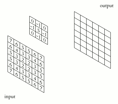
A Quick Note on Kernels

Before getting into the algorithms, it is worth explaining what a kernel is since both Sobel and Canny use them internally. A kernel is a small matrix, typically 3×3 or 5×5, that slides across the image one pixel at a time. At each position it multiplies its values against the corresponding pixels underneath and sums the results. This operation is called convolution, and depending on what numbers the kernel contains, it can produce very different effects: blurring, sharpening, detecting horizontal edges, detecting vertical edges, and so on.

When you passed a kernel size to cv2.GaussianBlur() in the previous post, you were controlling exactly this: how large a neighborhood of pixels gets factored into the blur at each position. Edge detectors use the same principle, but with kernels designed to respond to intensity changes rather than averages.

Sobel: The Gradient Directly

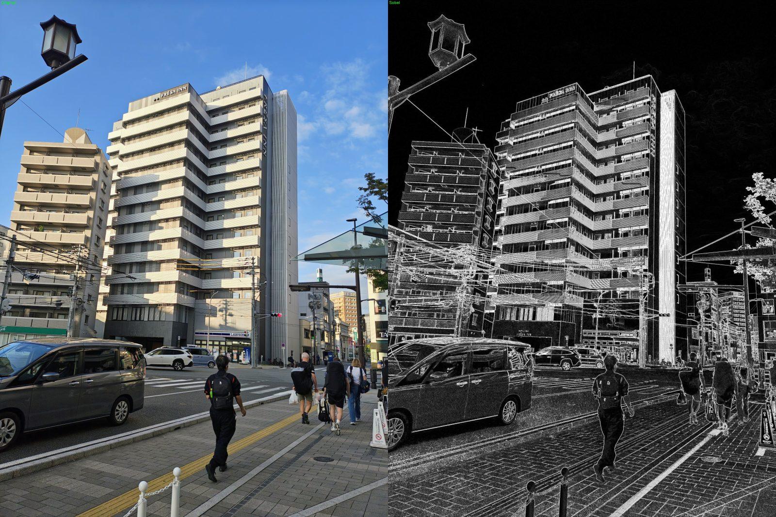
The Sobel operator is one of the simplest edge detectors. It computes the gradient in the horizontal and vertical directions separately by convolving the image with two small kernels. The result tells you not just where edges are but which direction they run.

The second argument cv2.CV_64F tells OpenCV to use 64-bit floats for the output. This matters because gradients can be negative, meaning intensity is decreasing, and if you use an unsigned 8-bit integer those negative values get clipped to zero and you lose half your edges. Computing in float and converting afterward keeps everything intact.

sobel_x responds strongly to vertical edges, transitions that run up and down. sobel_y responds to horizontal edges. Combining them with cv2.magnitude() gives the overall edge strength at each pixel regardless of direction.

Sobel is useful when you need directional information or want fine-grained control over the gradient computation. For most general-purpose edge detection though, Canny is the better tool.

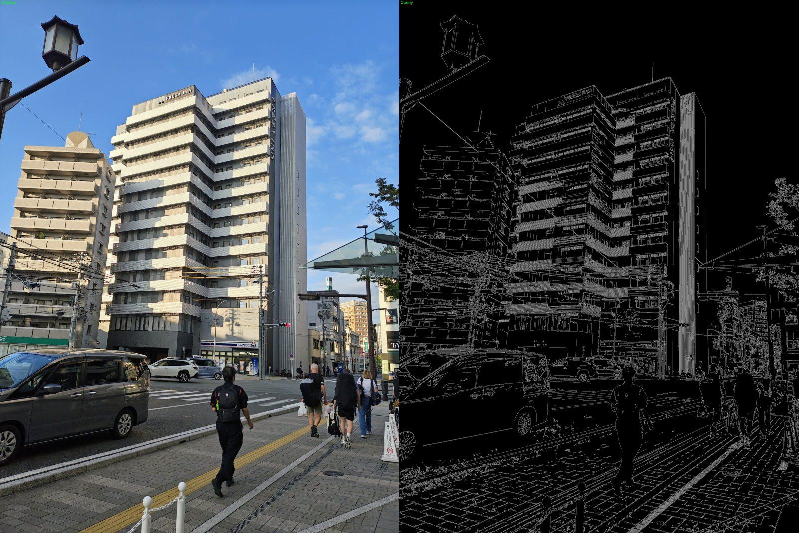
Canny Edge Detection

The Canny edge detector, developed by John Canny in 1986, is still the go-to choice for the vast majority of applications. What makes it better than a raw gradient threshold is its pipeline of steps: it smooths the image first to suppress noise, computes the gradient using Sobel internally, then applies non-maximum suppression to thin the detected edges down to single-pixel-wide lines, and finally uses a two-threshold system to decide which edges are real and which are not. The result is clean, thin, well-defined edges.

Applying a blur before Canny is good practice even though Canny does some smoothing internally. On noisy images the external blur makes a noticeable difference in how clean the output looks. A small kernel like (3, 3) or (5, 5) is usually enough.

The two numbers passed to cv2.Canny() are the low and high thresholds. Any gradient above the high threshold is a strong edge and is kept unconditionally. Any gradient below the low threshold is discarded. Anything between the two is kept only if it is connected to a strong edge. This hysteresis approach is what prevents Canny from producing scattered, fragmented results.

Canny also requires a grayscale image as input. Running it on a BGR image will not crash but it will not behave correctly. Always convert first.

Tuning the Thresholds

There is no formula that gives you the right thresholds automatically. It depends on the image, the lighting, the level of detail you care about, and what you are trying to detect. The honest answer is that threshold tuning is trial and error.

A good starting point is a 1:3 ratio between low and high, so (50, 150) or (100, 300). From there the logic is simple: if you are getting too many edges, noise and texture being picked up alongside real boundaries, increase both values. If you are missing edges or getting fragmented lines, decrease them. The ratio between the two matters more than the absolute numbers.

On images where you have direct control over the input, like a fixed camera in a controlled environment, it is worth spending time finding values that work well and locking them in. On arbitrary images from the wild, you will often find that no single pair of values works consistently across the full range of conditions, and that is a signal that threshold tuning alone is not enough and you need to look at preprocessing too.

Practical Tips

Lighting matters a lot. Edge detectors are sensitive to how contrast varies across the image. An evenly lit image will give you clean, consistent edges. Harsh shadows or uneven illumination will produce strong edges where you do not want them and miss edges where you do. If you are working with images from a controlled environment, fixing the lighting at the source is almost always worth more than any amount of threshold tuning.

Blurring kernel size affects detail. A larger kernel removes more noise but also smooths out fine edges. If you are losing edges that should be there, try a smaller blur or skip it entirely. If you are picking up too much texture and noise as edges, increase the kernel size.

Edge detection works best when there is a clear task. Running Canny on an arbitrary photo will give you a lot of edges, most of them uninteresting. The technique shines when you have a specific type of boundary you care about and you can tune the parameters and preprocessing for that specific case.

Wrapping Up

Edge detection is the first real analysis step in a computer vision pipeline. Before this, everything we did transformed images. Now we are extracting information from them. That is a different kind of operation and it opens up a different class of problems you can tackle.

In the next post we will take the output of edge detection and go one level further, grouping edges into shapes and extracting structured information about what is in the image.

See you in the next one.

Reference: Canny, J. (1986). A Computational Approach to Edge Detection. IEEE Transactions on Pattern Analysis and Machine Intelligence, Vol. 8, No. 6, pp. 679-698.