Fine Tuning a Pretrained Model with Hugging Face: A Hands On Guide

    This is a hands on tutorial on how to fine tune a pretrained model using Hugging Face. Instead of going over the theory in the abstract, we will work through one complete, real example from start to finish: taking DistilBERT and fine tuning it to detect toxic text. By the end you will have a saved, working classifier, and you will understand what every part of the code is doing and why.

    I picked toxicity detection because it is a simple binary classification problem, which makes it easy to follow, but the steps involved are exactly the same ones you would use for sentiment analysis, spam detection, intent classification, or pretty much any other text classification task. Once you understand this pipeline, you can reuse it for your own dataset with only small changes.

Why fine tuning instead of training from scratch

    Training a language model from scratch requires enormous amounts of data and compute, resources that most of us simply do not have lying around. Fine tuning takes a different approach. You start from a model that has already learned a rich representation of language from pretraining on massive text corpora, and you adapt that representation to your specific task using a comparatively small labeled dataset.

    DistilBERT, the model we will use here, is a smaller and faster version of BERT, built using a technique called distillation, where a smaller model is trained to mimic a larger one. It keeps most of BERT’s language understanding while being lighter and quicker to train, which makes it a solid pick for this tutorial since you can run the whole thing without needing heavy hardware.

The task and the dataset

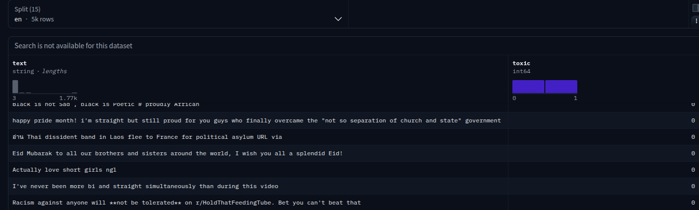
    We will use the textdetox multilingual toxicity dataset, restricted to the English split. Each example is a short piece of text paired with a binary label, 0 for non-toxic and 1 for toxic. This is a straightforward binary sequence classification problem, which is exactly why it makes such a good teaching example. Once you understand this pipeline, you can point it at almost any labeled text dataset and get a working classifier.

    Before jumping into code, it helps to have the full picture in your head. Fine tuning a transformer for classification with Hugging Face generally involves these six stages:

1. Load the dataset and split it into training, validation, and test sets
2. Tokenize the text so the model can read it
3. Load a pretrained model with a classification head attached
4. Define how you will measure performance
5. Configure and run the training loop
6. Save the fine tuned model so you can reuse it later

    Let’s go through each one.

Setting up and loading the data

    The Hugging Face datasets library gives you a single function, load_dataset, that can pull data directly from the Hugging Face Hub. No manual downloading, no writing a custom parser, it just works.

    Two small details here matter more than they look. First, we only load the en split, since the dataset is multilingual and we want to keep this example focused. Second, we rename the toxic column to label. This is not cosmetic. The Hugging Face Trainer expects a column called label by default, and if your dataset uses a different name, training will fail with a fairly cryptic error. Renaming it up front saves you a debugging session later.

    Next we split the data into training, validation, and test sets. Most datasets on the Hub only ship with a single split, so this part is usually on you.

    The numbers here can look confusing at first, so it helps to break down what each split is for:

• Training set, 70 percent of the data. This is what the model actually learns from during gradient updates. It needs to be the largest chunk since this is where all the actual learning happens.
• Validation set, 20 percent of the data. Used during training to check how the model performs on unseen data after every epoch. This is what lets us pick the best checkpoint and notice overfitting while it is still happening, instead of finding out too late.
• Test set, 10 percent of the data. Touched exactly once, after training is completely finished. This gives an honest, unbiased estimate of real world performance. If you peek at the test set repeatedly while tuning hyperparameters, it quietly turns into a second validation set and stops being a fair measurement.

Tokenizing the text

    Transformers do not read text the way we do. They operate on numerical token ids, so raw strings need to be converted before they can be fed into the model. That conversion has to match exactly what the model saw during pretraining, which is why we always load the tokenizer published alongside the model instead of writing our own.

    A few things worth noting. AutoTokenizer automatically figures out which tokenizer implementation matches distilbert-base-uncased, so you never have to know the underlying details. truncation=True makes sure any text longer than the model’s maximum sequence length gets cut down rather than causing an error. Setting batched=True speeds things up considerably, since the tokenizer processes many examples at once instead of one at a time. We also drop the original text column afterwards, since the Trainer only needs numeric tensors from here on.

    Notice we did not pass a fixed padding length to the tokenizer. That is intentional. Instead of padding every example in the dataset up front to the same length, which wastes memory on batches full of short sentences, DataCollatorWithPadding pads dynamically, batch by batch, only as much as the longest sequence in that particular batch requires. It is a small optimization but it adds up over a full training run.

Loading the model

    This single line does more than it looks like. AutoModelForSequenceClassification loads the pretrained DistilBERT weights, then attaches a fresh classification head on top, a simple linear layer that maps the model’s internal representation to num_labels output scores. Since this dataset is binary, toxic or not toxic, we set num_labels=2. That new head starts out randomly initialized, since it did not exist during pretraining, which is exactly why the whole model needs to be fine tuned rather than used as is.

    This is also a good moment to notice how little of this pipeline is actually specific to DistilBERT. The Auto classes exist precisely so you can swap the MODEL_NAME string for practically any model on the Hugging Face Hub and the rest of the code keeps working unchanged. You could drop in bert-base-uncased, a multilingual model like xlm-roberta-base, or even a much larger decoder based model such as Gemma or Llama 3.2, since AutoModelForSequenceClassification supports those architectures too by attaching the same kind of classification head on top.

Defining how success is measured

    The Trainer does not know what “good performance” means unless you tell it. We do that with a compute_metrics function, which the Hugging Face evaluate library makes easy to set up.

    During evaluation the model outputs raw logits, one score per class, rather than clean predictions. np.argmax picks the class with the highest score for each example, giving us the model’s actual predicted label. We then compare those predictions against the ground truth using accuracy as the metric. Accuracy works fine here since the classes are not heavily imbalanced, but for problems with severe class imbalance you would usually reach for precision, recall, or F1 instead, since accuracy alone can be misleading in those cases.

Configuring training

    TrainingArguments is the control panel for the whole run. output_dir is where checkpoints and logs get written. Setting both eval_strategy and save_strategy to epoch means the model gets evaluated and saved after every full pass through the training data, which keeps things easy to reason about.

    Batch size and epoch count are hyperparameters you will often tune for your own hardware and dataset. A batch size of 16 is a safe default that fits comfortably on most modern GPUs, and three epochs is typically enough for fine tuning, since the model already has strong language understanding from pretraining. The learning rate of 2e-5 is a well established starting point for fine tuning BERT style models, small on purpose, so we nudge the existing representations toward the new task instead of overwriting them.

    The last two arguments are easy to miss but matter a lot. load_best_model_at_end, combined with metric_for_best_model="accuracy", tells the Trainer to track validation accuracy across epochs and automatically reload the best checkpoint once training finishes, rather than leaving you with whatever the last epoch happened to produce, which is not always the best one. report_to="none" just keeps this example self contained, in a real project you would likely point it at something like Weights and Biases or TensorBoard.

Putting it together with the Trainer

    The Trainer class ties every piece together, the model, the training configuration, the datasets, the tokenizer, the data collator, and the metric function. Once trainer.train() runs, it handles the entire loop for you, batching, forward passes, loss computation, backpropagation, optimizer steps, evaluation, and checkpointing, without you writing a manual training loop.

    After training finishes, we call trainer.evaluate() again, this time on the held out test set. This is the number that actually matters for judging production performance, since the model has never seen this data during training or during any validation based decisions.

Saving the fine tuned model

    Saving only the model without the tokenizer, or the other way around, leaves you with something awkward to reload correctly later. Saving both together in the same directory means you can load the whole thing back with a single from_pretrained call, whether that is a few minutes later in the same script or months later in a different project. This same directory structure is also exactly what you would push to the Hugging Face Hub if you wanted to share the model publicly.

Wrapping up

    What we walked through here is a complete, production reasonable fine tuning pipeline, not a stripped down toy example. Load and split your data, tokenize it, load a pretrained model with the right number of output labels, define your metric, configure the Trainer, and save the result. That pattern applies almost unchanged whether you are building a toxicity filter, a sentiment classifier, a spam detector, an intent classifier, or pretty much any other text classification system you can think of.

    And because everything here is built on the Auto classes, the pipeline is not tied to DistilBERT at all. Change the MODEL_NAME variable and you can fine tune BERT, RoBERTa, a multilingual model, or even a large modern model like Gemma or Llama 3.2, using the exact same code. If you want to take this further, a natural next step is running the saved model through the pipeline function for quick inference, or trying a larger base model if accuracy on your test set is not quite where you need it. Either way, the core workflow you now understand carries over directly.

Full code

    If you just want the whole script in one place to copy and run, here it is.