OpenCV with Python: How Images Are Represented in Computer Vision

How Images Are Represented in Computer Vision

In the last post, we installed OpenCV and loaded some images… But if you just copy and paste code without knowing what is actually going on underneath, you will hit a wall pretty fast. So before we move on to doing more interesting things, let us talk about what an image actually looks like from a computer’s point of view.

When we look at a photo, we see colors, shapes, depth, context. A computer sees none of that. It does not “see” anything in any meaningful sense. What it gets is a matrix of numeric values, and everything that computer vision does, detecting faces, reading road signs, identifying tumors, is built on top of operations applied to those numbers. The visual meaning is something we layer on top afterward.

So: an image is a big grid of numbers. That is genuinely all it is. Once that sinks in, a lot of things in this field start to click.

The Array Behind OpenCV Images

When OpenCV reads an image with cv2.imread(), what you get back is a NumPy array. NumPy is a Python library for numerical computation, and the good news is you do not need to install it separately, it comes along automatically when you install OpenCV. Its main data structure is the ndarray, short for n-dimensional array. Think of it as the generalized version of the arrays you already know: a 1D array is just a list of numbers, a 2D array is a table of numbers with rows and columns, and a 3D array stacks multiple tables on top of each other. Images slot right into that model.

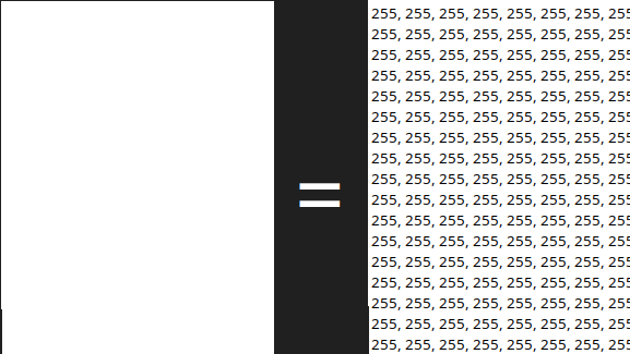
A grayscale image is a 2D array. Every element is a number from 0 to 255, where 0 is black, 255 is white, and everything in between is some shade of gray.

A color image is a 3D array. Each pixel carries three values, one for each color channel. This follows the RGB model: Red, Green, Blue. The reasoning behind it is that almost any color the human eye can see can be reproduced by mixing those three primaries at different intensities. Each channel goes from 0 to 255, so a pixel that is (255, 0, 0) in RGB is pure red, (0, 255, 0) is pure green, and (0, 0, 255) is pure blue. Mix them and you get everything else.

So a color image becomes a 3D array: height, width, and 3 channels. Try it yourself:

You will see something like (480, 640, 3). That is 480 rows, 640 columns, and 3 channels. Multiply those together and a single regular photo is already close to a million individual numbers. For the image below for instance, you’ll see (351, 600, 3).

BGR, Not RGB

Here is the thing that trips up pretty much everyone at some point. OpenCV does not store channels in RGB order. It stores them as BGR: Blue first, then Green, then Red. This goes back to how certain hardware and older codecs laid out pixel data back when the library was first built, and it just stuck.

The practical problem is that most other tools, Matplotlib, web browsers, deep learning frameworks, they all expect RGB. So if you load an image with OpenCV and hand it directly to one of those, the colors come out wrong. If you need to convert to RGB before passing it somewhere else, it is one line:

Worth keeping in the back of your head. Unexplained blue tints or weird skin tones are usually this.

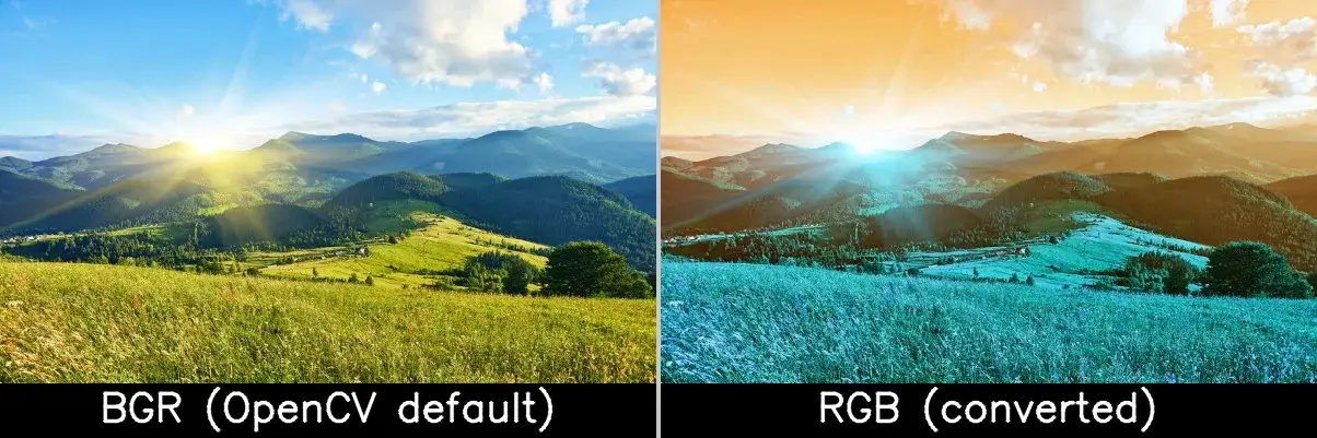
The image below makes this concrete. Both sides are the same file. The left one is the original BGR image saved directly by OpenCV, which knows it is BGR and handles it correctly. The right one was converted to RGB first and then saved by OpenCV, which re-interpreted those RGB values as BGR and swapped the channels again, producing the bluish result.

Accessing Images and Modifying Pixels

Since the image is just an array, you index into it like any other NumPy array using image[row, column]. Rows go from top to bottom, so row 0 is the very top of the image. Columns go from left to right, so column 0 is the left edge. That means image[0, 0] is the top-left pixel, and image[479, 639] on a 480×640 image is the bottom-right. For a color image, each pixel gives you back three values in BGR order:

You can write to pixels the same way. To set a pixel to pure red, remember BGR so red is the last channel:

And NumPy lets you operate on entire regions in one shot, no loops needed. This paints a 50×50 block black:

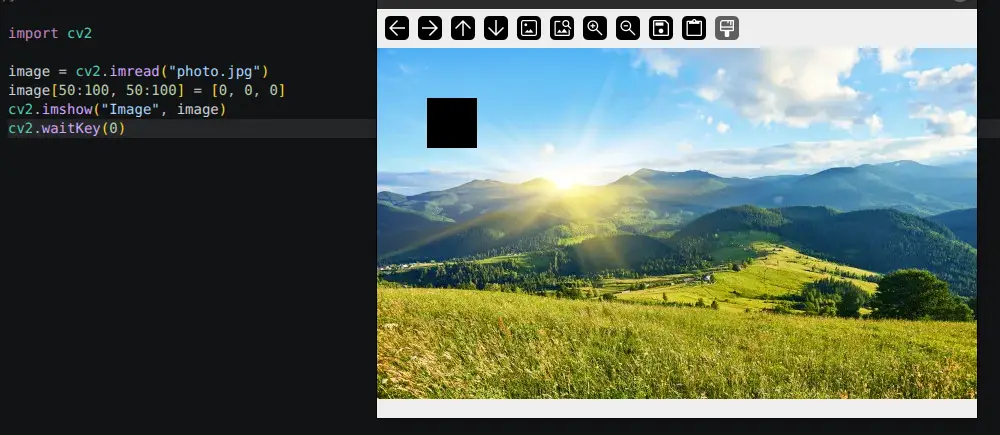
This is a big deal in practice. Looping over millions of pixels in Python would be painfully slow. Working with NumPy slices, it is nearly instant.

Converting Images to Grayscale

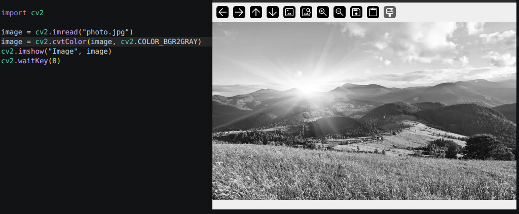
A lot of classic computer vision algorithms work on grayscale images, and not simply because of memory or speed. Many of them are designed around intensity, which is how bright or dark a region is, rather than hue. Edge detection, for example, looks for sharp transitions in pixel values. Thresholding separates foreground from background based on brightness. In those cases, color is not just unnecessary, it can actually get in the way. Grayscale strips out the information that does not contribute and keeps the signal the algorithm actually cares about. The conversion itself is one line:

The shape goes back to 2D. Each pixel ends up as a single value computed from a weighted mix of the original R, G, and B channels. The weights are not equal because human vision is more sensitive to green than to red or blue, so the formula reflects that. You do not need to deal with the math directly, cv2.cvtColor() handles it, but it is good to know it is not just a plain average.

Wrapping Up

To summarize what to carry forward: a color image in OpenCV is a NumPy array of shape (height, width, 3), values from 0 to 255, channels in BGR order. A grayscale image is (height, width), one value per pixel. Every algorithm you will ever run on an image is, at the end of the day, just math on those numbers.

This is the mental model you will carry through everything else in this series. Whenever something behaves unexpectedly, whether it is a wrong color, a failed detection, or a shape mismatch, come back to the array. Nine times out of ten the answer is there.

See you in the next one.